Cost Modeling for Cloud Applications: A Quick Guide using Jupyter Notebooks
By Michael Olson | Principal Software Engineer
Introduction
When building a cloud application, it’s important to understand the costs associated with the cloud services you’re using. This can help you make informed decisions about how to optimize your application for cost efficiency as well as prevent unexpected costs from cropping up over time. Traditional tools offered by cloud providers often fall short in giving the depth of insight needed across the lifecycle of cloud infrastructure. This guide explores how Jupyter Notebooks can be employed to create custom cloud cost models that offer a deeper understanding of spending, reveal cost drivers, and help in designing a scalable, efficient cloud architecture.
Benefits of Custom Modeling
There are a number of benefits in creating a cost model that is customized to your cloud architecture.
- Input assumptions like user count, fleet size, and data volume allow for tuning the model, ensuring flexibility and accuracy across different scenarios.
- Custom models help developers break down costs by features, services, or items, pinpointing expense drivers and identifying cost-saving opportunities.
- Grouping spend by cloud application features aids in determining the necessity of high-cost features.
- Custom models reveal hidden costs in managed services, offering transparency and debunking myths about these expenses.
- Coding custom models enables the use of APIs for real-time pricing data, improving forecast accuracy and model efficiency.
Creating a Cost Model with Jupyter Notebooks
Diving deeper into the practicalities, let’s explore how to build a cloud cost model using Python and Jupyter Notebooks. As we go through this example there will be a few helper functions that will be referenced in the code snippets. A complete version of this example can be found in this GitHub repository.
Cloud Architecture
For this example we will be modeling the following AWS architecture for real-time data ingest from a fleet of IoT devices:
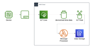
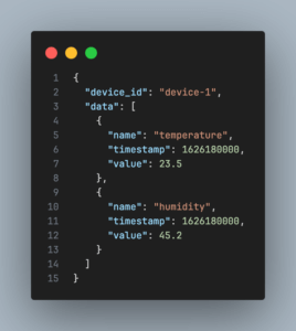
Devices publish data to an MQTT broker, which triggers an IoT Topic Rule to invoke a Lambda function. The Lambda function processes the data and writes it to a DynamoDB table. Each device will report an array of measurements with a timestamp and value. An example of the data format is shown below:
For this example we have a few cost drivers to consider:
- Messages processed by the MQTT broker
- IoT Topic Rule executions
- Lambda function runtime
- DynamoDB writes and storage
Assumptions
Starting out with the model we will need to make some assumptions around the inputs to the model. Let us assume the following:
- Fleet size: 10,000 devices
- Messages per device: 10 messages per minute
- Message size: 2 KB
- Lambda function runtime: 1500ms
- DynamoDB record size.
- Record lifetime: 180 days
Installing Dependencies
To get started, we will first need to install the necessary Python packages. For this example I will be using the poetry package manager to create a virtual environment and manage dependencies. We’ll need the following packages:
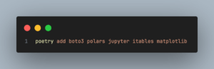
For this example we will use the pola.rs for composing and manipulating cost data, but you can also use Pandas if you are more comfortable with that data analysis library.
Retrieve Pricing Data
We could manually input the prices into our notebook for everything. This is easier, but experience has taught us that these prices tend to get out-of-date fairly quickly. It is a bit more work up-front to automate the price retrieval, but we have found this to be worth the effort.
The AWS SDK (boto3) provides a simple way to fetch pricing data for AWS services. We can use this to retrieve the pricing information for the services we will be using in the cloud. The following code snippets demonstrate how to fetch the desired service pricing as a pola.rs DataFrame.
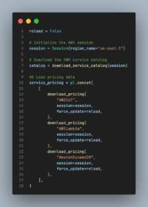
This code block instantiates the boto3 session, downloads the service catalog and then downloads the needed pricing information as a pola.rs data frame. The service codes used when downloading pricing actually come from the service catalog, which is downloaded to the “cache” folder in the project directory. So if you need info for additional services that is where to find the necessary code.
Composing the Model
Now we have what we need to compose the cost model. We’ll break the model down into these main features:
- Fleet
- Device Messaging
- Message Processing
- Data Storage
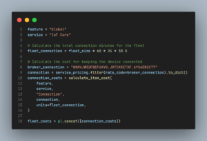
Let’s start with modeling the costs related to the device fleet. The main cost driver here will be persisting a connection to the MQTT broker in IoT Core which is charged in the number of connection minutes. The following code snippet demonstrates how to calculate the costs for the device fleet.
The next feature to model is device messaging. There a few cost drivers to consider here:
- The number of messages the MQTT broker processes
- The number of topic actions
- The number of executions by the rules engine
For all three of these we will need to calculate the total number of messages sent by the fleet. The following code block demonstrates how to calculate the costs for device messaging.
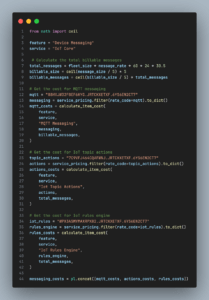
Note: AWS charges per message up to 5KB. If a message is larger than 5KB it is considered to be two messages.
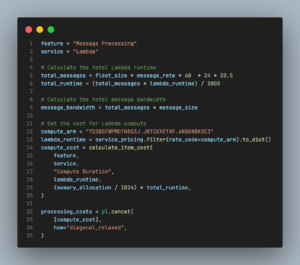
Up next is the compute resources needed to process the incoming messages. The code block below shows how to calculate the cost for Lambda Function execution.
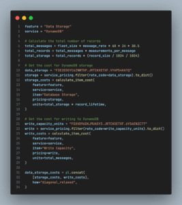
Lastly we need to model the costs related to writing and storing the data in DynamoDB. The code block below demonstrates how to calculate the costs for data storage.
Displaying the Results
With all of the architecture and cost assumptions in place, we can now run the model and display the results. The code below demonstrates how to calculate the total cost for the architecture and display the results in an interactive table.
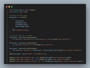
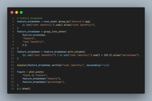
Now it is all well and good to have the total costs, but what if we want to see how the costs are distributed across the various features? Since all the cost data is in a dataframe we can easily break resource costs down to the feature / service / item level. The code below shows how to aggregate costs into the desired grouping and display the results as a pie chart.
As modeled, the total cloud costs for this architecture would be:
- Total Cost (Monthly): $22,257.98
- Total Cost (Yearly): $267,095.70
- Total Cost (Device Lifetime): $267.10
And the costs per feature / service / item breakdown as follows.
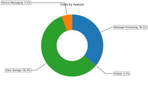
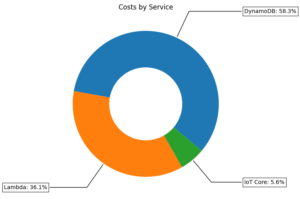
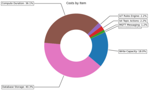
So we can see that the main cost drivers for our cloud architecture are Lambda function runtime and data storage.
Refining the Model
Now that we have a working model of our cloud architecture we can use it to refine the design of the cloud. As modeled the cost processing and storing device measurements are the biggest drivers for cloud spend so it raises a question, “Do we need that much data”? What if we reduced the time resolution so that devices were to send 10 messages an hour instead of 10 per minute. This simple change drops cloud spend from around $22k per month down to $400.
Conclusion
Through this example we’ve walked through the creation of a customized cost model using code and Jupyter Notebooks. We’ve also shown some of the benefits of going through this exercise vs using more traditional tools. If you need help with cost estimations or optimizing your cloud spend, don’t hesitate to reach out to us.